RabbitFarm

The standard way that graphs are taught in Prolog is to represent the graph edges in the Prolog database and then, as needed, manipulate the database using assertz/1 and retract/1. There really is nothing wrong with this for many applications. However, when dealing with large graphs the overhead of writing to the database may not be worth the performance gain (via indexing) when querying. Especially in cases when the amount of querying may be low, there may not be any “return on investment”.

An alternative method, promoted by Markus Triska, is the use of attributed variables. In this way a variable represents a graph node and the attributes represent edges. Additionally, beyond that basic representation, additional attributes can be used for other information on the node and to add attributes to the edges such as a weight or other information on the relationship between nodes.

To be clear, attributed variables are primarily intended for use when building libraries, such as for constraint logic programming. There the default Prolog unification algorithm is less convenient than an extended version using attributed variables. In these cases hooks are used to determine, say, domain constraints on variables. Here will not concern ourselves with such advanced topics!

Not all Prologs provide attributed variables. Scryer and SWI are among those that do. All of our code is implemented and tested using SWI-Prolog.

Examples

Let’s start off with the most basic example: a small set of otherwise meaningless nodes connected at random.

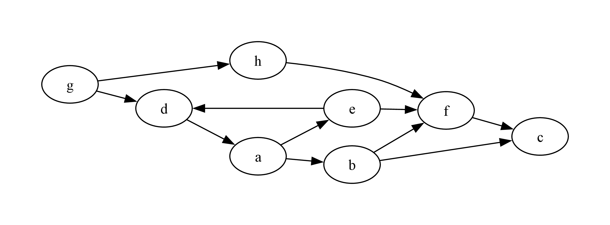
This small graph, adapted from an example in Clocksin’s Clause and Effect, can be represented in Prolog in the traditional way as follows.

As needed additional edges can be added and removed from the Prolog database dynamically using assertz/1 and retract/1.

How might we change this to an attributed variables representation?

First off, we need to keep in mind that only an uninstantiated variable can have an attribute set unless we also provide an attribute hook. Since we otherwise have no need for a hook, we will restrict ourselves to having only uninstantiated variables as nodes. Of course, we need to maintain information for each node and edge. In both cases the node information and the edge information are kept as attributes. At first this sounds more complicated than it really is. Let’s see how it comes together in practice.

To build a bridge from the old to the new we will first create a predicate, edges_attributed/2 which converts a list of edges (e.g. [edge(a, b), edge(b, f), edge(f, c)]) to a list of attributed variables where the edges are attributes on the nodes. The attributes on each node are a list of edges to other node and, also, an attribute containing the node label.

For now we are only concerning ourselves with simple graphs like the example, so nodes are just unique atoms (e.g. a, b, c, ...). We’re also assuming that all edges are directed as given.

A lot of work is happening in helper predicates via maplist/3. For the most part these are just one or two lines each.

The lengthiest of the predicates used in a maplist/3 is graph_attributed/3. This is where the final assembly of the graph of attributed variables takes place.

Testing this predicate out, with just a small set of edges, we can get a sense of this new representation. A weight attribute, with default value of 1, has been added to demonstrate the possibility of attributed edge variables, but we won’t make any further use of this here.

?- Edges = [edge(a, b), edge(b, c), edge(b, d)], 
edges_attributed(Edges, Attributed). 
Edges = [edge(a, b), edge(b, c), edge(b, d)], 
Attributed = [a-_A, b-_B, c-_C, d-_D], 
put_attr(_A, node, a), 
put_attr(_A, edges, [edge(_E, a-_A, _B)]), 
put_attr(_B, node, b), 
put_attr(_B, edges, [edge(_F, b-_B, _C), edge(_G, b-_B, _D)]), 
put_attr(_C, node, c), 
put_attr(_C, edges, []), 
put_attr(_D, node, d), 
put_attr(_D, edges, []), 
put_attr(_E, weight, 1), 
put_attr(_F, weight, 1), 
put_attr(_G, weight, 1).

That looks nice, but let’s put it to work with a basic traversal.

To start with, let’s defines a predicate to determine if any two nodes are connected by a directed edge. If one or both of the two node arguments are uninstantiated then member/2 will find one for us, otherwise this will just confirm they are in the Graph, which we will be passed to all predicates that need it. This small amount of extra bookkeeping is part of the trade-off for no longer using the dynamic database.

Also, speaking of extra bookkeeping, we’ll try and maintain a level of encapsulation around the use of attributed variables. For example, in the following predicates we only need worry about the handling of attributes when determining connectedness. When building on this code for more complex purposes that is an important part of the design to keep in mind: encapsulate the low level implementation details and provide predicates which have a convenient higher level of interface.

In the spirit of building a big example, the following code does the same connectedness check, but for undirected edges. We’re not worrying too much about such graphs, but this is one way to do it.

Finally we can use this connectedness check to define path finding predicates that look a lot like any standard Prolog example of path finding you may have seen before!

Closing

At this point you should understand how to build a graph using attribute variables in Prolog. The example code here can be further extended as needed. You’ll find that this approach can take on quite a good deal of complexity!

All the code above is structured in a single file as shown. A link to this is in the References section.

Indices

Files

"graph.p" Defined by 14.

Fragments

⟨ Construct a graph of attributed variables. 6 ⟩ Referenced in 2.

⟨ Convert list of edges to attributed variables. 2 ⟩ Referenced in 14.

⟨ Create a K-V pair for each node. 8 ⟩ Referenced in 14.

⟨ Create a unique list of nodes. 4 ⟩ Referenced in 2.

⟨ Determine if two nodes are connected by a directed edge. 11 ⟩ Referenced in 14.

⟨ Determine if two nodes are connected by an undirected edge. 12 ⟩ Referenced in 14.

⟨ Example Graph (Standard) 1 ⟩ Referenced in 14.

⟨ Extract the nodes from all edges. 3 ⟩ Referenced in 2.

⟨ Find a path between any two nodes, if such a path exists. 13 ⟩ Referenced in 14.

⟨ From the node pairs, create the graph of attributed variables. 10 ⟩ Referenced in 14.

⟨ Generate attribute edge list. 9 ⟩ Referenced in 14.

⟨ Helper predicate for extracting nodes from edges. 7 ⟩ Referenced in 14.

⟨ Make the list of K-V pairs for the nodes. 5 ⟩ Referenced in 2.

References

This method has been promoted by Markus Triska on Stack Overflow, but publicly available examples are rare. Hopefully this page will be useful to any interested persons looking for more information.

Stack Overflow Post #1

Stack Overflow Post #2

Strongly Connected Components An implementation of Tarjan’s strongly connected components algorithm which uses this graph representation.

graph.p